h. Workforce
- Daniel Olivera (Unlicensed)
- Anonymous
 Workforce
Simulation
This tool is useful to make Staffing, that is to know how many agents are needed in my Contact Center to answer calls, also it is interesting to make ForeCasting estimating the volume of growth of the Contact Center to know how many agents are going to be needed to reach those desired metrics of Service Level and Abandon.
Erlang
The Erlang distribution is a two parameter family of continuous probability distributions  y
y 
- a positive integer 'shape'
- a positive real 'rate' ; sometimes the scale
 , the inverse of the rate is used.
The density function for values  is
is
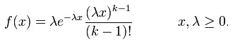
The Erlang distribution with shape parameter equal to 1 simplifies to the exponential distribution. It is a special case of the Gamma distribution. It is the distribution of a sum of independent exponential variables with mean each.
Are good for Staffing, know how many agents I need in my Contact Center also is great for ForeCasting using the metrics of Service Level and abandon rate.
Erlang C
Consider the classic M/M/c queueing model: Poisson arrival process, exponential service time and no abandonment by the customers (that is, customers have infinite patience time). The queue capacity can be finite or infinite. Because there are no abandonment's, the number of servers must be greater than the offered load for the queue to be stable and reach steady state. Let λ be the arrival rate and 1/μ the average waiting time, then the offered load is ρ=λ/μ.
Performance
- Service level (SL): This measure is defined as the expected ratio of customers that waited less or equal to the acceptable waiting time t. That is t
SL(y,t )=𝔼[X (y,t )]/𝔼[A] - Where y is the number of agents, X(y,t) is the number of customers that waited at most t as a function of y and t, A is the total number of customers, and 𝔼 is the expected value operator in statistics.
- Wait probability: The probability that a new customer will have to wait in queue. This is also equal to the proportion of customers that join the waiting queue.
- The average waiting time of a customer.
- Service level (SL): This measure is defined as the expected ratio of customers that waited less or equal to the acceptable waiting time t. That is t
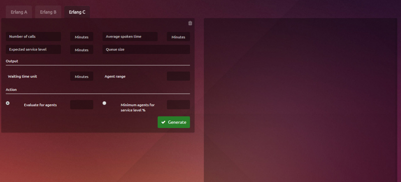
Parameters
- Number of calls: The average number of customers that arrive per time unit. For example, 5.7 customers per minute.
- Average spoken time: The average time duration that an agent takes to serve one customer. For example, an average service time of 10.5 minutes per customer.
- Expected Service Level (Max wished): This is the waiting time threshold of the service level (SL) measure. For example, the acceptable waiting time can be 20 seconds.
- Queue size: The maximum size of the waiting queue. When the queue is full, all new customers are blocked. This parameter must be integer. Set a negative value to choose an unlimited queue capacity. For better algorithm efficiency, we recommend to set an unlimited capacity rather than an arbitrary large number.
- Waiting time unit: Select the time unit of the average waiting time results.
- Agent range: Allows to evaluate multiple agents. Example, 5 and evaluate for 10 agents, so will have data between 5 and 15 agents.
- Evaluate for agents:Allows to evaluate the performance measures for multiple number of agents.
- Minimum agents for service level %: Find the minimum number of servers required to attain a service level (SL) equal or higher than the given SL target.
For example, set this parameter to 80 and the Service Level to 20 seconds to find the minimum number of servers needed for a service level of at least 80% with a waiting time threshold of 20 seconds..
Example:
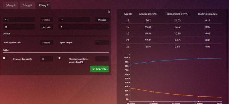
Charts
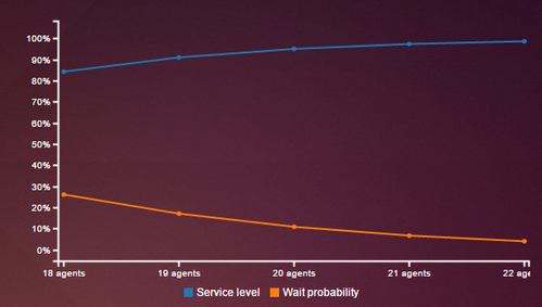
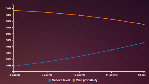
1) Service Level, Wait Probability
The chart show the probability that has a client in enter a queue and the behavior of the Service Level for those Agents.
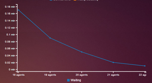
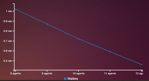
2) Wait
The chart shows the mean of wait for the clients including abandon and answered for those Agents.
Erlang A
Consider the following M/M/c+M queueing model: Poisson arrival process, exponential service time and exponential patience time. This queueing system is always stable because of customer abandonment's. Also due to abandonment's, there are different ways to account the customers that abandoned in the service level (SL) function.(SL1 and SL2) for the SL and one approximate formula (SLD) based on diffusion equations. The choice of an exact or approximate SL formula will also decide on whether this program will use the exact or approximate formulas for the other performance measures (abandonment ratio, delay probability and average waiting time).
Performance
- Service Level (SL): The ratio of customers that wait t or less to be served:
- SL1: The customers that abandoned but waited at most t are excluded from the service level. SL1(y,t )=𝔼[X (y,t )] / 𝔼[A−G(y,t )]
- SL2: The customers that abandoned but waited at most t are counted as having received a "good" quality of service. SL2(y,t)=E[X(y,t)+G(y,t)] / E[A].
- SLD: An approximation of SL2 based on diffusion equations. This formula is taken from the paper of Garnett, Mandelbaum and Reiman (2002).
SL1 ≤ SL2.
For high traffic use SLD. - Wait Probability: The probability that a new customer will have to enter the waiting queue because all servers are busy. This is also equal to the proportion of customers that join the waiting queue.
- Abandon rate: The proportion of customers that abandoned the queue without receiving service.
- Average waiting time: The average waiting time of a customer (including served and abandoned customers).
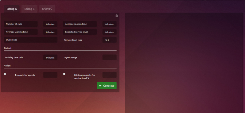
Parameters
- Number of calls: The average number of customers that arrive per time unit. For example, 5.7 customers per minute,
- Average spoken time: The average time duration that an agent takes to serve one customer. For example, an average service time of 10.5 minutes per customer.
- Average waiting time:The average time duration that a customer is willing to wait in the queue. For example, an average of 5.2 minutes per customer.
- Expected Service Level (Max wished): This is the waiting time threshold of the service level (SL) measure. For example, the acceptable waiting time can be 20 seconds.
- Queue size: The maximum size of the waiting queue. When the queue is full, all new customers are blocked. This parameter must be integer. Set a negative value to choose an unlimited queue capacity. For better algorithm efficiency, we recommend to set an unlimited capacity rather than an arbitrary large number.
- Type service level: SL1, SL2, SLD.
- Waiting time unit: Select the time unit of the average waiting time results.
- Agent range: It allows multiple measures to evaluate agents. Example, 5 and is evaluated for 10 agents, so we will have data between 5 to 15 agents.
- Evaluate for agents:Allows to evaluate the performance measures for multiple number of agents.
- Minimum agents for service level %: Find the minimum number of servers required to attain a service level (SL) equal or higher than the given SL target.
For example, set this parameter to 80 and the Service Level to 20 seconds to find the minimum number of servers needed for a service level of at least 80% with a waiting time threshold of 20 seconds..
Example:
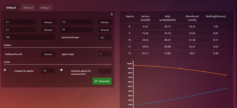
Charts
1) Service Level and Wait Probability
The chart show the probability that has a client in enter a queue and the behavior of the Service Level for those Agents.
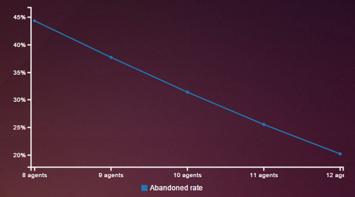
2) Abandon rate
Percentage of clients without agent.
3) Wait
The chart shows the mean of wait for the clients including abandon and answered for those Agents.
Erlang B
We assume the classic M/M/c queueing model with Poisson arrival process, exponential service time and no queueing capacity. That is, any new customer that sees all agents busy at their time of arrival will be blocked from the system and forced to abandon. The number of states in the system is equal to: number of servers + 1 (empty state). With a minimum of 1 agent, this queueing system is always stable, because there is no waiting queue. All non-blocked customers are automatically served and their waiting time is 0.
Abandon Probability
This measure is defined as the probability that all agents are busy in the queueing system when a new customer arrives. This is also equal to the proportion of time that all agents are busy.
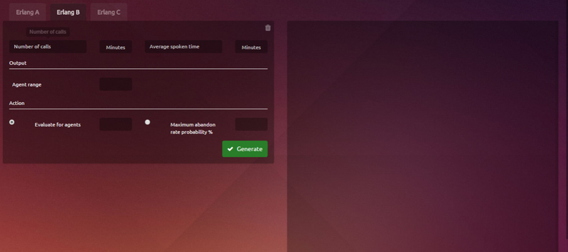
Parameters
- Number of calls: The average number of customers that arrive per time unit. For example, 5.7 customers per minute.
- Average spoken time: The average time duration that an agent takes to serve one customer. For example, an average service time of 10.5 minutes per customer.
- Agent range: It allows multiple measures to evaluate agents. Example, 5 and is evaluated for 10 agents, so we will have data between 5 to 15 agents.
- Evaluate for agents:Allows to evaluate the performance measures for multiple number of agents.
- Max Abandon rate probability: Find the minimum number of servers, let's say Y, required to have a blocking probability equal or less than the maximum blocking threshold. Let B(y) be the blocking probability as a function of the number of servers y, and T the maximum blocking threshold. Y =min{y:B(y)≤T ,y∈ℕ} Example 5 to find the abandon rato of a max of 5% Abandon.
Example:
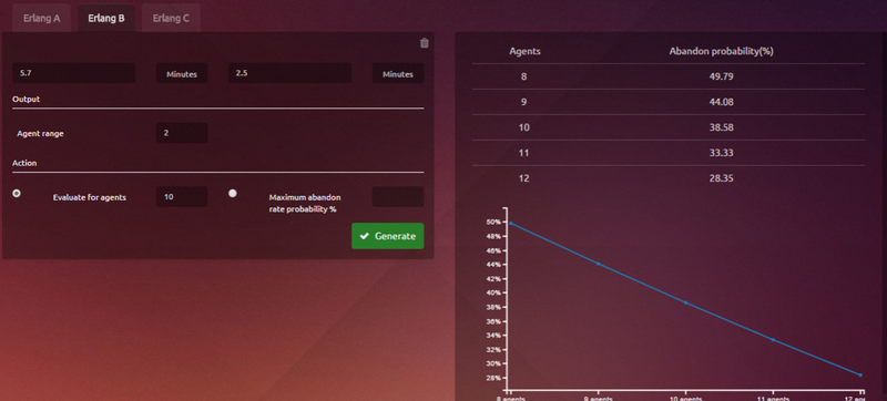
Charts
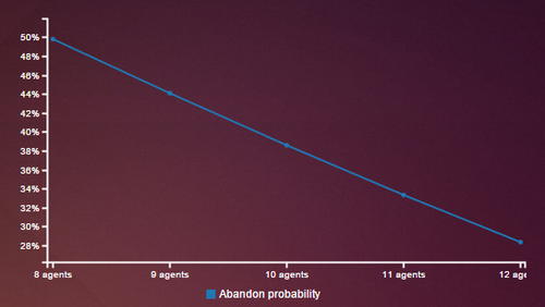
1) Abandon rate
Probability of all agents busy when a new customer arrives.